Wide DHMPC DLRC

Synthesis of Networked Switching Linear Decentralized Controllers

The purpose of the DLR is to synthesize a decentralized feedback gain that is capable of robustly stabilize a linear plant while enforcing a set of constraint on input and state variables under the effect of unknown but bounded disturbances. The synthesis is carried out by solving a semi-definite programming problem, SDP, which can efficiently be solved by means of linear matrix inequalities, LMI.

A detailed description of the used procedure is available in "D. Barcelli, D. Bernardini, and A. Bemporad, “Synthesis of networked switching linear decentralized controllers” in Proc. 49th IEEE Conf. on Decision and Control, Atlanta, GA, USA, 2010, pp. 2480–2485."

Plant Description

The linear plant is modeled as discrete-time time-invariant linear system as

x(t + 1) = Ax(t) + Bu(t)

where $x = {[x_1,\ldots,x_n]}{'} \in \mathbb{R}^n$ is the state, $u = {[u_1,\ldots,u_m]}{'} \in \mathbb{R}^m$ is the input and $A \in \mathbb{R}^{n \times n}$, $B \in \mathbb{R}^{n \times m}$. We assume that states and inputs are subject to the constraints $\|x(t)\|_2\leq x_{\max},\ \|u(t)\|_2\leq u_{\max},\ \forall t\in\mathbb{N}_0.$

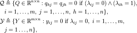
The process we consider is a networked control system, where spatially distributed sensor nodes provide measurements of the system state, and spatially distributed actuator nodes implement the control action. More in detail, at every time step t every sensor $s_1,\ldots,s_n$ measures a component x_i(t) of the state vector, $i=1,\ldots,n$. Then, measurements are sent to actuators $a_1,\ldots,a_m$ through a user-defined networked connection. Given a process we define its \emph{network topology} by means of an adjacency matrix $\Lambda\in\{0,1\}^{m\times n}$ with elements

$\lambda_{ij} = \left\{ \begin{array}{ll} 1 & \mbox {if sensor } s_j \mbox{ is ideally linked to actuator } a_i,\\ 0 & \mbox{otherwise.} \end{array} \right.$

for $i=1,\ldots,m$ and $j=1,\ldots,n$. In other words, λ_ij = 1 if and only if the measurement x_j(t) can be exploited to compute the input signal u_i(t), $\forall t\in\mathbb{N}_0$.

Our goal is to find a gain matrix $K\in\mathbb{R}^{m\times n}$ such that the system in closed-loop with

u(t) = Kx(t)

is asymptotically stable. The desired control law must be decentralized, i.e., each actuator $a_1,\ldots,a_m$ can only exploit the measurements that are available in accordance with the network topology. In other words, each row i of K can only have non-zero elements in correspondence with the state measurements available to actuator a_i, $i=1,\ldots,m$. This imposes the following structure on K:

$\lambda_{ij}=0 \ \Rightarrow\ k_{ij} = 0, \ \ i=1,\ldots,m, \ j=1,\ldots,n,$

where k_ij is the (i,j)-th element of K.

An usual technical trick is to synthesize the controller K as K = YQ ^{− 1}, where $Y \in \mathbb{R}^{m \times n}, Q \in \mathbb{R}^{n \times n}$ are the solution of the following SDP problem:

$\begin{align} \min_{\gamma,Q,Y} &\;\; \gamma\\ s.t. &\; \left[\begin{smallmatrix} Q & \star & \star & \star \\ AQ+BY & Q & \star & \star \\ Q_x^{1/2}Q & \mathbf{0} & \gamma I_n & \star \\ Q_u^{1/2}Y & \mathbf{0} & \mathbf{0} & \gamma I_m \end{smallmatrix}\right] \succeq0,\\ &\; \left[\begin{smallmatrix} Q & \star \\ AQ+BY & x_{\max}^2I_n \end{smallmatrix} \right]\succeq0, \\ &\; \left[\begin{smallmatrix} u_{\max}^2I_m & \star \\ Y & Q \end{smallmatrix} \right]\succeq0, \\ &\; \left[\begin{smallmatrix} 1 & \star \\ v_i & Q \end{smallmatrix} \right] \succeq0,\ i=1,\ldots,n_v,\\ &\; Y\in\mathcal{Y},\ Q\in\mathcal{Q}, \end{align}$

where I_n is the identity matrix in $\mathbb{R}^{n\times n}$, $\mathbf{0}$ is a matrix of appropriate dimension with all zero entries,

$\begin{align} \mathcal{Q} &\triangleq \{ Q\in\mathbb{R}^{n\times n} : q_{hj}=q_{jh}=0 \mbox{ if } (\lambda_{ij}=0) \wedge (\lambda_{ih}=1), \\ & i=1,\ldots,m,\; j=1,\ldots,n,\; h=1,\ldots,n \}, \\ \mathcal{Y} &\triangleq \{ Y\in\mathbb{R}^{m\times n} : y_{ij} = 0 \mbox{ if } \lambda_{ij}=0,\ i=1,\ldots,m, \\ & j=1\ldots,n \}, \end{align}$

and q_ij, y_ij are the (i,j)-th elements of Q and Y, respectively. Finally$\mathbb{X}_0$ is the set of all admissible initial conditions.

Robust Switching Controllers

To account for not ideality of links we extend the definition of the adjacency matrix Λ as 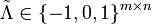$\tilde \Lambda\in\{-1,0,1\}^{m\times n}$ with elements

$\tilde \lambda_{ij} = \left\{ \begin{array}{ll} 1 & \mbox {if sensor } s_j \mbox{ is ideally linked to actuator } a_i,\\ -1 & \mbox {if sensor } s_j \mbox{ is faulty linked to actuator } a_i,\\ 0 & \mbox{otherwise.} \end{array} \right.$

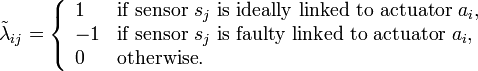
Such extension allow to model some sensor-to-actuator connections which are subject to packet dropouts. This complicates the control problem as none of the actuators is aware of which measurement are exploitable for the current instant feedback computation.

Uncertain entries in Λ are such that the aforementioned structure of K must hold accordingly to the current losses occurrence. That implies that each controller cannot use the measurements which it did not received. Moreover, each controller is only aware of its losses occurrence, which implies that it must compute its feedback independently on the other controller measurements status. It follows that the usable state components for the generic i-th controller gain, given a losses configuration, is determined only by the configuration of its variables. For a more detailed description we refer to the paper.

The aforementioned SDP is then reformulated accounting for all losses possible configurations, and not reported here for brevity.

The robust design account for the worst case realization and guarantees stability while enforcing constraints for any occurrence of losses. Such technique is the sole capable of strict constraint enforcement, but its is relatively conservatives as it ignores possible information available for the losses distribution.

Stochastic Switching Controllers

In order to reduce the conservatism introduced by the Robust Controller, assume a realistic model of the packet dropouts among the network, which is the probability distribution of the network configurations $\{\tilde\Lambda_h\}$ is modeled by a finite-state Markov chain with 2 states, called Z₁ and Z₂.

The dynamics of the Markov chain are defined by a transition matrix

$T = \left[\begin{array}{cc}q_1 & 1-q_1\\ 1-q_2 & q_2\end{array}\right]$

such that $t_{ij}=\Pr[z(t+1)=Z_j \,|\, z(t)=Z_i]$, and by an emission matrix $E\in\mathbb{R}^{2\times2^L}$ such that $e_{ij}=\Pr[\tilde\Lambda(t)=\tilde\Lambda_j \,|\, z(t)=Z_i]$, being t_ij and e_ij the (i,j)-th element of T and E, respectively. In order to define the values in E we need to compute the probabilities of occurrence of $\tilde\Lambda_h$, $\forall h$. We assume that the occurrence of a packet dropout at a time step t in a given network link is an i.i.d. random variable, for every state of the Markov chain. In particular, we denote with d₁ and d₂, 0 < d₁ < d₂ < 1, the probabilities of losing a packet at time t if z(t) = Z₁ and z(t) = Z₂, respectively (for example, in Z₁ we have "few" dropouts, and in Z₂ we have "many", according to Gilbert's model). Moreover, let s_1,h and s_0,h be the total number of lossy links in Λ which are mapped as ideal links and as no links in $\tilde\Lambda_h$, respectively, i.e.,

$\begin{align} s_{1,h} &= \sum_{(i,j)\in\mathcal{I}}\tilde\lambda_{ij}^h,~~~ h=1,\ldots,\ell,\\ s_{0,h} &= \sum_{(i,j)\in\mathcal{I}}(1-\tilde\lambda_{ij}^h),~~~ h=1,\ldots,\ell, \end{align}$

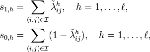
where $\mathcal{I}\triangleq\{(i,j)\in\{1,\ldots,m\}\times\{1,\ldots,n\} : \lambda_{ij}=-1\}$. Then, we can define the elements {e_ij} of E as

$e_{ij} = {d_i}^{s_{0,j}}{(1-d_i)}^{s_{1,j}},\ i=1,2,\ j=1,\ldots,\ell.$

As detailed on the paper, this method cannot guarantee stability while enforcing constraints in a strict sense, but in the so called mean-square sense. In the current frame work such definition is equivalent to

$\lim_{t\to\infty} \mathbb{E}\left[{\|x(t)\|}^2\right]=0.$

which is to allow the Lyapunov function to occasionally increase in two consecutive steps, provided that the converging condition as well as constraints hold on average. That is to allow point-wise constraint violation, but hopefully for a short period of time, while most of the time constraints are enforced. In practical cases it usual to "estimate" some constraints, in the sense that the threshold value is set by means of engineering insight only and not basing on a real physic law. In those occasions to allow minor violation is very likely to not be a problem at all, and this latter approach allow to achieve better performances for such small price to pay.

Class Description

The inputs for the class are

• the network state, i.e. the connection matrix of each node to each actuator;
• the matrices A and B modeling the controlled plant dynamics;
• the weights for the Riccati equation;
• the state and input constraints;
• the polytope mapping the initial state uncertainty (given as a set of vertices).
• the Markov chain modeling packet dropouts (needed for stochastic stability only)

All the methods solve an SDP problem and provide a feedback matrix gain K, and the matrix solution of the Riccati equation P. The SDP problems are dependent on the type of stability required. These methods are:

• Centralized: the network is assumed fully connected, all links are reliable and faultless (i.e., no packet dropouts are considered);
• Decentralized Ideal: the network is only partially connected, all links are reliable and faultless;
• Decentralized Robust: the network is only partially connected, and some links are faulty, i.e., packets transmitted in those links can be lost. This method provides a decentralized controller that guarantees stability for any possible configuration of packet drops, while robustly fulfilling state and input constraints;
• Decentralized Stochastic: the network is only partially connected, and some links are faulty, i.e., packets transmitted in those links can be lost. Dropouts are modeled by a Markov chain and closed-loop stability is guaranteed in the mean square sense. This solution is intended to be less conservative with respect to the robust one.

Output (read-only) properties

Mc is a structure which defines the Markov chain. It includes:

• T : transition matrix;
• E : emission matrix.

The other properties are the output of the SDP solution:

• P : solution of Riccati equation;
• K : feedback matrix gain (i.e. u=K*x);
• g : γ in P = γQ ^{− 1} that is the minimized parameter in the SDP optimization;

Each of the previous properties is a structure with fields:

• ci : centralized ideal;
• di : decentralized ideal
• dl : decentralized lossy, i.e. robust;
• ds : decentralized stochastic. that are computed by corresponding methods.

Class Methods

Class constructor

obj=decLMI(Net,A,B,Qx,Qu,X0,xmax,umax,Mc);

Net : matrix of row size equal to number of actuators and columns size equal to number of states. Net(i,j) can be: 1 : if the state j is connected to actuator i by an ideal link;0 : if there is no link between state j and actuator i;-1: if the state j is connected to actuator i by a lossy link;

A : state matrix of the LTI system modeling the plant;

B : input matrix of the LTI system modeling the plant;

Qx : state weight matrix of the Riccati equation;

Qu : input weight matrix of the Riccati equation;

X0 : set of vertices of the polytope that defines the uncertainty of the initial state condition;

xmax : Euclidean norm constraint on state;

umax : Euclidean norm constraint on input;

Mc : two-states Markov chain that models the probability of losing a packet. Must be a structure with fields:

• d : array, where d(i) is the probability of losing a packet being in the i-th state of the Markov chain;
• q : array, where q(i) is the probability of remaining in the i-th state of the Markov chain.

Centralized LMI computation

obj = obj.solve_centralized_lmi();

Computes the solution of the SDP problem assuming the network to be fully connected and each link completely reliable. The goal is to give a reference for the performances that can be achieved via the decentralized methods.

Decentralized Ideal computation

obj = obj.solve_dec_ideal_lmi();

Computes the solution considering only present links, but assuming that all of them are reliable. Basically does not account for miss-reception of packets containing measurements.

Decentralized Robust computation

obj = obj.solve_dec_lossy_lmi();

Computes a decentralized controller which provides stability and constraints satisfaction for any possible occurrence of the packet dropouts.

Decentralized Stochastic computation

obj = obj.solve_dec_stoch_lmi;

Computes a decentralized controller that exploits the available knowledge on the dropouts probability distributions. A two-states Markov chain is used to model the packet losses. Mean-square stability is guaranteed.

[Wide main page]